Introduction

Convolutional Neural Networks (CNNs) are the foundation of modern Computer Vision. From identifying faces in photo galleries to helping autonomous vehicles navigate busy streets, CNNs are a powerful subset of Deep Learning that enables machines to interpret visual data.

Although the mathematics behind CNNs can become complex, the architectural logic is surprisingly intuitive. At their core, CNNs are built around three essential steps.

The Three Mandatory Steps of a CNN

Every CNN architecture is built upon three primary layer types.

1. The Convolutional Layer

This layer acts as the "eyes" of the network and is responsible for feature extraction.

Input

For a standard RGB image, the input contains three dimensions:

• Width
• Height
• Depth (RGB channels)

The Convolution Process

The convolutional layer uses a filter (also called a kernel), which slides across the image like a moving window.

As it moves, the filter performs mathematical operations to detect patterns such as:

• Edges
• Curves
• Shapes
• Textures

For example, the network may learn to identify:

• The edge of a cat's ear
• The whiskers of a cat
• Fur textures

Result

The output is called a feature map (or activation map), which highlights where certain features were detected in the image.

2. The Pooling Layer (Max-Pooling)

Feature maps generated by convolution layers can become very large.

Pooling layers reduce spatial dimensions, making computation more efficient while also helping prevent overfitting.

Max-Pooling

In max-pooling, a small window (commonly 2×2) slides across the feature map.

For each window, only the maximum value is preserved.

Example:

[1 3]
[2 9]

Becomes:

9

This preserves the strongest signals while discarding weaker or noisy information.

3. The Fully Connected (FC) Layer

Once features are extracted and compressed, they are passed into a traditional dense neural network.

Structure

Every neuron in this layer is connected to every neuron in the previous layer.

Classification

The fully connected layer performs the final classification step using activation functions such as Sigmoid.

Example:

0.95

This would represent a 95% probability that the image belongs to a specific class (e.g., a cat).

Essential Mathematics: Functions for Learning

To transform raw image data into meaningful predictions, CNNs rely on several mathematical functions.

1. Activation Functions

Activation functions introduce non-linearity into the network, allowing it to learn complex patterns instead of simple linear relationships.

Sigmoid Function

The Sigmoid function behaves like a smooth switch, compressing values between 0 and 1.

Formula:

σ(x) = 1 / (1 + e^(-x))

Derivative:

σ'(x) = σ(x)(1 - σ(x))

ReLU (Rectified Linear Unit)

ReLU is the most commonly used activation function for hidden layers.

Rule:

f(x) = max(0, x)

Meaning:

• Positive values remain unchanged
• Negative values become 0

Derivative:

1 if x > 0
0 otherwise

ReLU is computationally efficient and helps mitigate vanishing gradient issues.

2. Loss Function (Binary Cross-Entropy)

The loss function measures how far the prediction is from the true label.

For binary classification tasks such as:

• Cat vs Not-Cat
• Spam vs Not-Spam

We commonly use Binary Cross-Entropy (BCE).

Formula:

L = -[y log(ŷ) + (1 - y) log(1 - ŷ)]

Where:

• y → true label
• ŷ → predicted probability

The lower the loss, the better the model performs.

The Training Loop: Backpropagation & Gradient Descent

The network learns by continuously adjusting its weights to reduce prediction error.

This process is called Backpropagation.

1. Backpropagation

The network computes gradients (derivatives) of the loss with respect to each parameter.

These gradients determine:

• Which direction to update the weights
• How large the update should be

2. Gradient Descent

The parameter update rule is:

θ = θ - α(∂L / ∂θ)

Where:

• θ → weights or biases
• α → learning rate
• ∂L / ∂θ → gradient of the loss

The learning rate controls how aggressively the model updates itself during training.

Architecture Overview

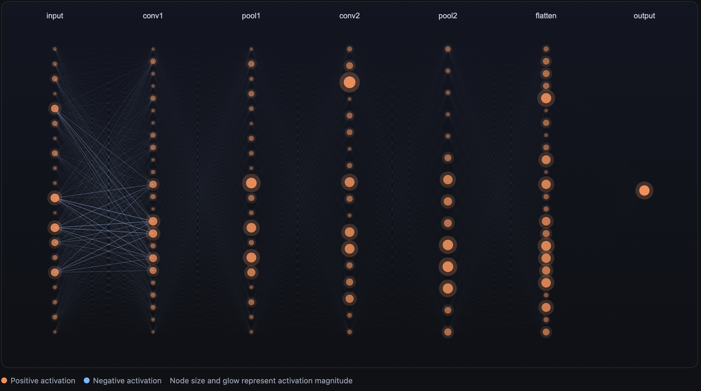
Putting it all together and to better understand these concepts, here is the architecture I implemented for my cat-cnn project.

CAT-CNN Architecture

Input Layer

64×64 grayscale image

Convolution Layer 1

3×3 kernel → 62×62 feature map

Max-Pooling Layer 1

2×2 pooling → 31×31 feature map

Convolution Layer 2

3×3 kernel → 29×29 feature map

Max-Pooling Layer 2

2×2 pooling → 14×14 feature map

Flatten Layer

The 2D feature maps are transformed into a 1D vector.

14×14 → 196 values

Dense Layer

196 inputs → 1 output neuron

Output Layer

A Sigmoid activation produces the final probability prediction.

Example:

0.92 → 92% probability the image contains a cat

CAT-CNN Training metrics

{
  "loss": 0.6810561289476712,
  "accuracy": 0.6555023923444976,
  "precision": 0.0,
  "recall": 0.0,
  "f1": 0.0,
  "tp": 0,
  "tn": 137,
  "fp": 0,
  "fn": 72,
  "samples": 209
}

Final Thoughts

Building a CNN from scratch was one of the most valuable learning experiences I have had in machine learning, a great way to understand how neural networks process images and progressively learn meaningful visual features.

This project also sparked a deeper interest in Deep Learning and Computer Vision, especially in understanding how mathematical operations translate into intelligent predictions. Thanks for reading, and I hope this article helped simplify the fundamentals of Convolutional Neural Networks.

If you would like to explore the implementation details and source code, feel free to check out the full project repository here.