Introduction

Linear Regression and Logistic Regression are among the foundational algorithms in Machine Learning. They introduce the core ideas behind prediction, optimization, and learning from data.

I recently explored these concepts and wanted to share my understanding in the simplest way possible, including:

• Mathematical intuition
• Practical applications
• Python implementation concepts

These techniques are simple, powerful, and an excellent starting point for anyone beginning their Machine Learning journey.

Linear Regression — Predicting Continuous Values

1. What Is Linear Regression?

Linear Regression is used to predict continuous numerical values by finding the straight line that best fits a dataset.

Examples include:

• Predicting house prices based on size
• Estimating exam scores from study hours
• Forecasting temperatures

The objective is to model the relationship between input variables and output values.

2. The Math Behind Linear Regression

The equation of a straight line is:

y = w·x + b

Where:

• y → predicted output
• x → input feature
• w → weight (slope)
• b → bias (intercept)

The model learns the optimal values of w and b during training.

3. Mean Squared Error (MSE)

To measure how good the predictions are, we use the Mean Squared Error (MSE) loss function.

Formula:

MSE = (1/n) Σ(yᵢ - ŷᵢ)²

Where:

• n → number of observations
• yᵢ → actual value
• ŷᵢ → predicted value
• (yᵢ - ŷᵢ)² → squared prediction error

The goal is to minimize this error.

4. Python Implementation from Scratch

A simple Linear Regression implementation can be built using:

• NumPy for numerical operations
• Gradient Descent for optimization
• Matplotlib for visualization

import numpy as np  # Importing NumPy, a library for numerical computations
import matplotlib.pyplot as plt  # Importing Matplotlib for plotting

# Example data: Study hours vs. Exam scores
X = np.array([1, 2, 3, 4, 5])  # Study hours, defined as a NumPy array for vectorized operations
y = np.array([50, 55, 65, 70, 80])  # Exam scores, also a NumPy array for compatibility with NumPy operations

# Initialize parameters
w = 0  # Initial weight (slope of the regression line), starts at 0
b = 0  # Initial bias (y-intercept of the regression line), starts at 0
learning_rate = 0.01  # Step size for gradient descent updates, controls how much parameters are adjusted per iteration
epochs = 1000  # Number of iterations to run the gradient descent optimization

# Gradient Descent
for epoch in range(epochs):  # Repeat the optimization process for a specified number of epochs
    y_pred = w * X + b  # Compute predicted values (y = wX + b) using current parameters
    error = y - y_pred  # Calculate the error between actual (y) and predicted (y) values

    # Compute gradients
    dw = -2 * np.sum(X * error) / len(X)  # Gradient of the loss with respect to w (partial derivative), derived from MSE formula
    db = -2 * np.sum(error) / len(X)  # Gradient of the loss with respect to b (partial derivative), derived from MSE formula

    # Update parameters
    w -= learning_rate * dw  # Update the weight using gradient descent rule: w = w - a * dw
    b -= learning_rate * db  # Update the bias using gradient descent rule: b = b - a * db

    # Optional: Print loss every 100 epochs
    if epoch % 100 == 0:  # Check if the current epoch is a multiple of 100
        mse = np.mean(error ** 2)  # Calculate Mean Squared Error (MSE) as the loss function
        print(f"Epoch {epoch}, MSE: {mse:.4f}")  # Print the epoch number and the corresponding MSE

# Final parameters
print(f"Final weight (w): {w:.4f}")  # Print the optimized weight after training
print(f"Final bias (b): {b:.4f}")  # Print the optimized bias after training

# Plot the data and regression line
plt.scatter(X, y, color='blue', label='Actual Scores')  # Plot actual data points as a scatter plot
plt.plot(X, w * X + b, color='red', label='Regression Line')  # Plot the regression line using optimized w and b
plt.xlabel('Study Hours')  # Label the x-axis as "Study Hours"
plt.ylabel('Exam Scores')  # Label the y-axis as "Exam Scores"
plt.legend()  # Add a legend to differentiate data points and the regression line
plt.show()  # Display the plot

# made by me @taha_boussaden
# you can also view my github: github.com/ThePhoenix77

# Date: 2024-11-28

Important Concepts

NumPy Arrays

np.array()

Used for efficient mathematical operations on vectors and matrices.

Gradients (dw and db)

The gradients are derived from the partial derivatives of the MSE loss function with respect to:

• w (weight)
• b (bias)

These gradients indicate how the parameters should change to reduce the loss.

Gradient Descent Updates

The parameters are updated using:

w = w - α·dw
b = b - α·db

Where:

• α → learning rate
• dw → derivative with respect to w
• db → derivative with respect to b

Visualization

Using:

plt.scatter()
plt.plot()

We can visualize:

• The original data points
• The regression line

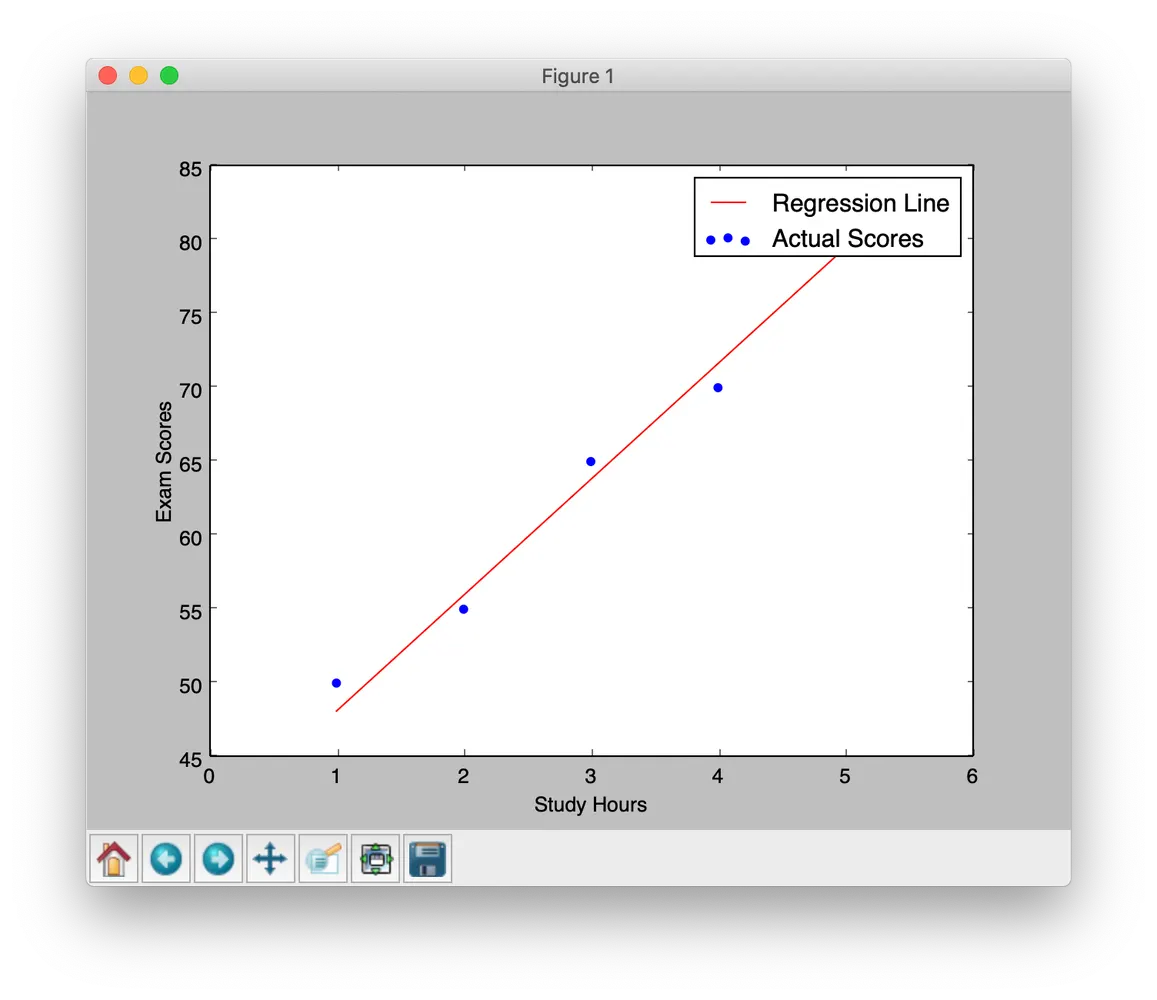
This helps understand how the model progressively learns the best fit.

Logistic Regression — Predicting Categories

1. What Is Logistic Regression?

Logistic Regression is used for classification problems where the output belongs to categories instead of continuous values.

Examples include:

• Cat vs Not-Cat classification
• Spam detection
• Predicting pass/fail outcomes
• Medical diagnosis

Despite the name, Logistic Regression is actually a classification algorithm.

2. The Math Behind Logistic Regression

Logistic Regression applies the Sigmoid Function to a linear equation.

First:

z = w·x + b

Then:

σ(z) = 1 / (1 + e^(-z))

The Sigmoid function converts values into probabilities between 0 and 1.

Example:

0.92 → 92% probability

I highly recommend visualizing the Sigmoid function graph, as it makes understanding its behavior much easier.

3. Binary Cross-Entropy Loss (BCE)

To evaluate predictions, Logistic Regression uses the Binary Cross-Entropy Loss function.

Formula:

L = -[y log(ŷ) + (1 - y) log(1 - ŷ)]

Where:

• y → true label (0 or 1)
• ŷ → predicted probability

This loss penalizes incorrect predictions more heavily when confidence is high.

4. Python Implementation from Scratch

A Logistic Regression model can also be implemented using:

• NumPy
• Sigmoid activation
• Gradient Descent

import numpy as np  # Importing NumPy for numerical computations

# Sigmoid function
def sigmoid(z):
    return 1 / (1 + np.exp(-z))  # Sigmoid activation function, maps input z to the range (0, 1)
    # Source: Logistic regression; used to model probabilities in binary classification.

# Binary Cross-Entropy Loss
def binary_cross_entropy(y, y_pred):
    return -np.mean(y * np.log(y_pred) + (1 - y) * np.log(1 - y_pred))
    # Binary Cross-Entropy (BCE) is a common loss function for binary classification.
    # Source: Derived from information theory, it measures the difference between actual labels (y) and predicted probabilities (y_pred).

# Example data: Hours studied vs Pass/Fail (1 = Pass, 0 = Fail)
X = np.array([1, 2, 3, 4, 5])  # Study hours, treated as features (input data)
y = np.array([0, 0, 1, 1, 1])  # Labels indicating Pass (1) or Fail (0)

# Initialize parameters
w = 0  # Initial weight (slope of the logistic model), starts at 0
b = 0  # Initial bias (y-intercept), starts at 0
learning_rate = 0.1  # Learning rate for gradient descent
epochs = 1000  # Number of iterations for optimizing the parameters

# Gradient Descent
for epoch in range(epochs):  # Perform optimization for a fixed number of epochs
    z = w * X + b  # Linear combination of features and weights (z = wX + b)
    y_pred = sigmoid(z)  # Apply sigmoid to compute predicted probabilities

    # Compute gradients
    dw = np.dot((y_pred - y), X) / len(X)  # Gradient of the loss with respect to w (partial derivative)
    db = np.sum(y_pred - y) / len(X)  # Gradient of the loss with respect to b (partial derivative)
    # Source of gradients: Derived from the BCE loss function.

    # Update parameters
    w -= learning_rate * dw  # Update weight using gradient descent rule
    b -= learning_rate * db  # Update bias using gradient descent rule

    # Optional: Print loss every 100 epochs
    if epoch % 100 == 0:  # Print every 100 iterations for monitoring progress
        loss = binary_cross_entropy(y, y_pred)  # Compute BCE loss for current predictions
        print(f"Epoch {epoch}, Loss: {loss:.4f}")  # Display the current epoch and loss

# Final parameters
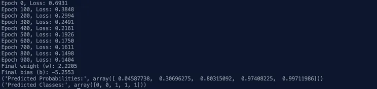
print(f"Final weight (w): {w:.4f}")  # Optimized weight after training
print(f"Final bias (b): {b:.4f}")  # Optimized bias after training

# Test predictions
z_test = w * X + b  # Linear combination for testing (same as training)
y_pred_test = sigmoid(z_test)  # Compute predicted probabilities for test data
predictions = (y_pred_test >= 0.5).astype(int)  # Convert probabilities to binary classes (threshold = 0.5)

print("Predicted Probabilities:", y_pred_test)  # Display predicted probabilities
print("Predicted Classes:", predictions)  # Display predicted classes (0 or 1)

# made by me @taha_boussaden
# you can also view my github: github.com/ThePhoenix77

# Date: 2024-11-28

Gradients (dw and db)

The gradients are derived from the partial derivatives of the BCE loss function.

These derivatives determine how much the parameters should change to minimize classification error.

Gradient Descent Updates

The update rule remains:

w = w - α·dw
b = b - α·db

Where:

• α → learning rate

Repeated updates progressively improve predictions.

Prediction Conversion

The output probability is converted into a binary class using a threshold.

Common rule:

ŷ ≥ 0.5 → predict 1
ŷ < 0.5 → predict 0

This transforms probabilities into final classifications.

Why and When to Use These Methods

1. Linear Regression

Use Linear Regression when predicting continuous numerical values such as:

• Prices
• Temperatures
• Sales
• Scores

2. Logistic Regression

Use Logistic Regression when solving classification problems such as:

• Disease prediction
• Email spam detection
• Image classification
• Fraud detection

Conclusion

When I first encountered Linear and Logistic Regression, I was surprised by how relatively simple mathematical equations could solve meaningful real-world problems.

Building these algorithms from scratch in Python helped me better understand:

• Optimization
• Gradient Descent
• Loss functions

These techniques are an excellent introduction to the AI world, especially Machine Learning.

If you are beginning your AI journey like me, I strongly recommend implementing these models manually before relying on high-level libraries. Understanding the fundamentals makes advanced concepts much easier later on.